Building a Protein Variant Classifier with ESM2 and Multi-GPU Training

Introduction

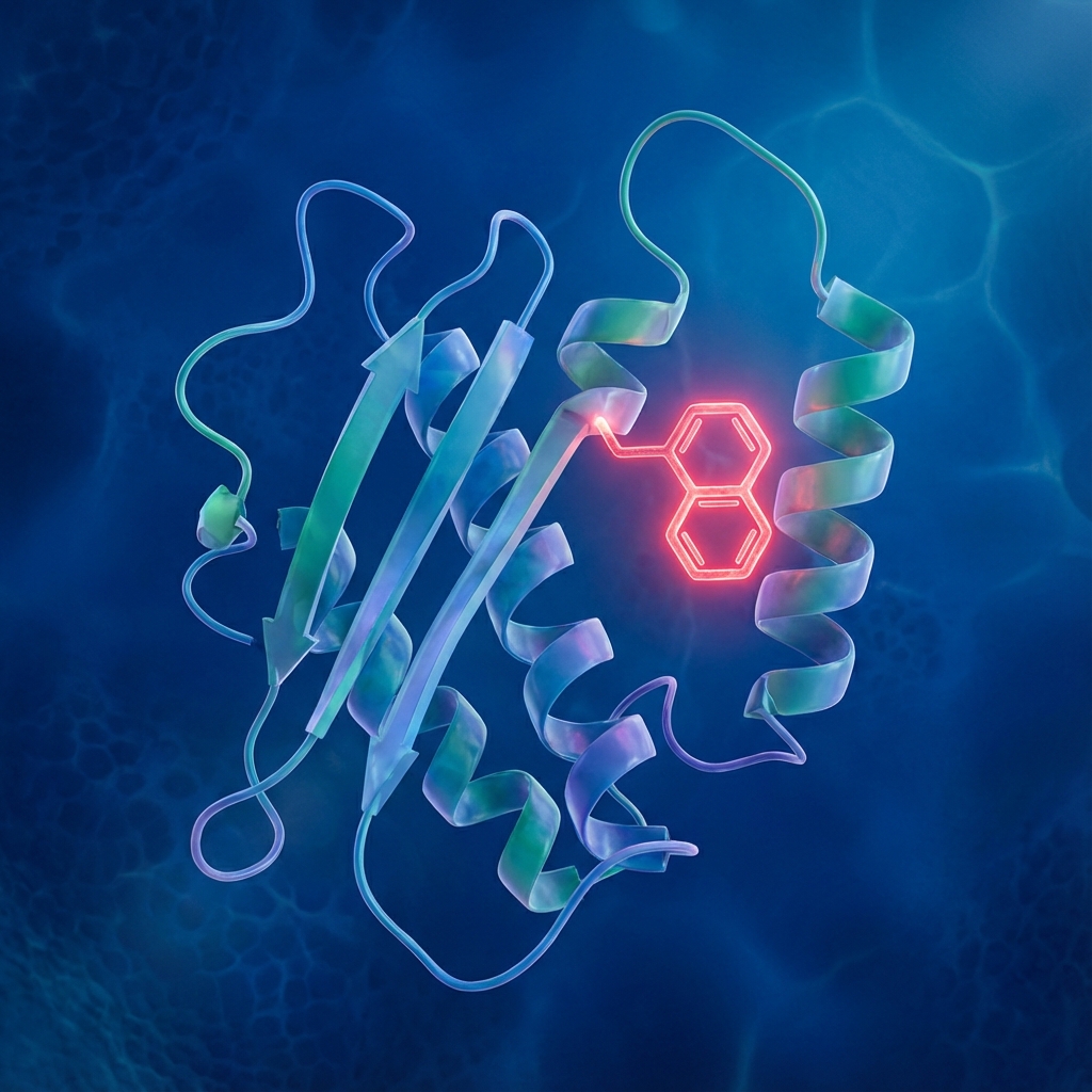
In the field of clinical genomics, accurately predicting whether a specific genetic variant is pathogenic (disease-causing) or benign is a critical challenge. Recently, I worked on a project to develop a deep learning model that classifies protein variants as either Gain-of-Function (GOF) or Loss-of-Function (LOF) using ESM2 (Evolutionary Scale Modeling), a state-of-the-art protein language model.

Challenge 1: Metric Selection for Clinical Use

Before diving into the model, I had to evaluate existing pathogenicity predictors. The dataset contains 107 patients, each with multiple variants where only a few are pathogenic (LABEL=1).

The Problem: Class Imbalance

The data is highly imbalanced—most variants are benign (LABEL=0), only a few are pathogenic (LABEL=1). This makes metric selection critical.

Metric	Formula	Problem with Imbalanced Data
Accuracy	(TP+TN) / Total	Predicting all as benign gives high accuracy
AUROC	Area under TPR-FPR curve	Can look good even with poor precision

Why AUROC Alone Is Not Enough

AUROC measures discrimination across all thresholds. A model with AUROC=0.94 sounds great, but:

• At what threshold does it achieve good Precision and Recall?
• In clinical diagnostics, False Negatives are dangerous (missing a pathogenic variant)

Metrics for Clinical Pathogenicity Prediction

For this problem, I focused on both classification metrics and ranking metrics:

Classification Metrics (Binary)

Metric	Formula	Clinical Importance
Recall (Sensitivity)	$\frac{TP}{TP + FN}$	Must be high: we cannot miss pathogenic variants
Precision (PPV)	$\frac{TP}{TP + FP}$	Reduces unnecessary follow-up tests
F1 Score	$\frac{2 \times Precision \times Recall}{Precision + Recall}$	Balances both for imbalanced data

Ranking Metric (Patient-Centric)

Since each patient has multiple variants and we want the pathogenic variant to be ranked high:

Metric	Formula	Clinical Importance
Top-K Recall	$\frac{\text{# patients with causal variant in top K}}{\text{# total patients}}$	Measures how often the pathogenic variant appears in the top K predictions

The formal definition:

\[\text{Top-K Recall} = \frac{1}{N} \sum_{i=1}^{N} \mathbb{1}[\text{rank}(v_i) \leq K]\]

Where:

• $N$ = number of patients
• $v_i$ = the pathogenic variant for patient $i$
• $\text{rank}(v_i)$ = position when variants are sorted by prediction score (descending)
• $\mathbb{1}[\cdot]$ = indicator function (1 if true, 0 if false)

Why Recall Is Critical

In medical diagnostics, a False Negative (predicting benign when actually pathogenic) means:

• Patient doesn’t receive treatment
• Disease progresses undetected

Therefore, Recall must be prioritized, even at the cost of some False Positives.

Evaluation Framework

I evaluated each predictor (A, B, C) with both classification and ranking metrics:

from sklearn.metrics import precision_recall_curve, roc_auc_score
import numpy as np

def evaluate_predictor(y_true: np.ndarray, y_scores: np.ndarray) -> dict:
    """Evaluate predictor with classification metrics."""
    auroc = roc_auc_score(y_true, y_scores)
    
    precisions, recalls, thresholds = precision_recall_curve(y_true, y_scores)
    f1_scores = 2 * (precisions * recalls) / (precisions + recalls + 1e-8)
    best_idx = np.argmax(f1_scores)
    
    return {
        "auroc": auroc,
        "best_f1": f1_scores[best_idx],
        "recall_at_best_f1": recalls[best_idx],
        "precision_at_best_f1": precisions[best_idx],
    }
# end def

def compute_top_k_recall(df: pd.DataFrame, score_col: str, k: int) -> float:
    """Compute Top-K Recall per patient."""
    hits = 0
    for patient_id, group in df.groupby("Patient_ID"):
        sorted_group = group.sort_values(score_col, ascending=False)
        top_k_labels = sorted_group.head(k)["LABEL"].values
        if 1 in top_k_labels:
            hits += 1
        # end if
    # end for
    return hits / df["Patient_ID"].nunique()
# end def

Results

Classification Metrics

Predictor	AUROC	Best F1	Recall @ Best F1	Precision @ Best F1
A	0.94	0.42	0.65	0.31
B	0.88	0.58	0.82	0.45
C	0.91	0.51	0.71	0.40

Ranking Metrics (Patient-Centric)

Predictor	Top-1 Recall	Top-5 Recall
A	12%	35%
B	24%	52%
C	18%	41%

Key Findings:

1. Predictor A had the highest AUROC but the worst F1, Recall, and Top-K metrics
2. Predictor B achieved 82% Recall and 52% Top-5 Recall—meaning it catches more pathogenic variants both in classification and ranking

Decision: For clinical use, Predictor B is preferred because:

1. Highest Recall (minimizes missed pathogenic variants)
2. Best F1 Score (balanced performance on imbalanced data)
3. Best Top-5 Recall (pathogenic variant is in top 5 for 52% of patients)

Lesson: In medical AI with class imbalance, evaluate using multiple metrics that reflect clinical consequences—not just AUROC.

Challenge 2: Modeling Protein Variants with ESM2

The core task was to classify variants using esm2_t33_650M_UR50D.

Existing vs. Proposed Approach

A standard approach in this domain often involves feeding the mutant sequence directly into the model to predict its property.

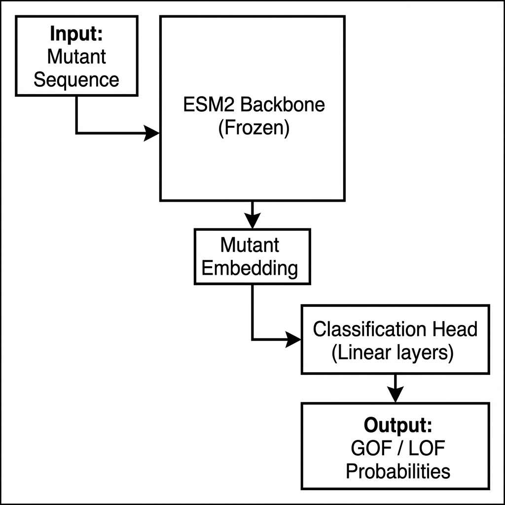Figure 1: Standard Baseline Approach. The model only sees the mutant sequence, making it difficult to learn the specific impact of the mutation relative to the wild-type.

However, simply feeding the mutant sequence isn’t enough. The model needs to understand what changed. I designed the input to explicitly capture the difference:

Input = Concat(E_wt, E_mut, E_mut - E_wt)

• E_wt: Embedding of the Wild-Type sequence
• E_mut: Embedding of the Mutant sequence
• Difference: The vector representing the direction of change (Mutant - Wild-Type)

This “Difference Vector” proved crucial for distinguishing between LOF (function loss) and GOF (function gain).

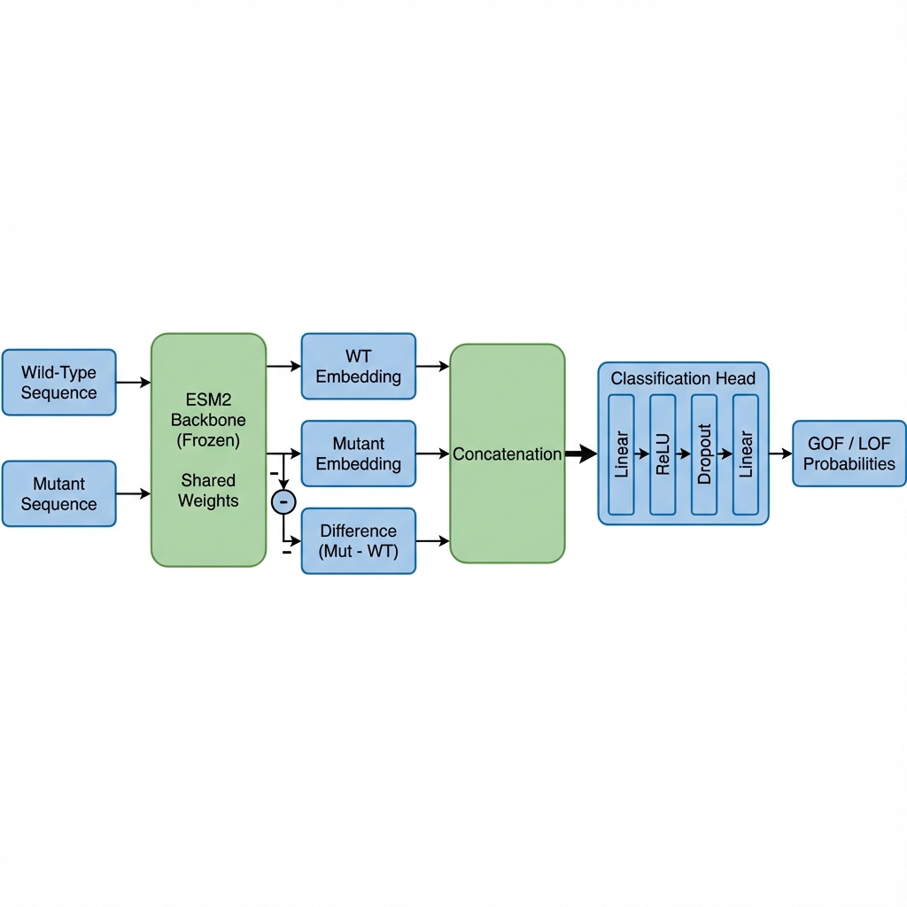Figure 2: Our Proposed Architecture. By explicitly feeding the difference vector (Mutant - WT), the model can directly focus on the functional shift caused by the variant.

Code Snippet: Model Architecture

class ESM2VariantClassifier(nn.Module):
    def __init__(self, model_name="facebook/esm2_t33_650M_UR50D"):
        super().__init__()
        self.esm = EsmModel.from_pretrained(model_name)
        # Freeze backbone for efficiency
        for param in self.esm.parameters():
            param.requires_grad = False
            
        hidden_size = self.esm.config.hidden_size
        
        self.classifier = nn.Sequential(
            nn.Linear(hidden_size * 3, 512), # 3x input size due to concatenation
            nn.ReLU(),
            nn.Dropout(0.3),
            nn.Linear(512, 2)
        )

    def forward(self, wt_ids, wt_mask, mut_ids, mut_mask):
        wt_out = self.esm(input_ids=wt_ids, attention_mask=wt_mask)
        mut_out = self.esm(input_ids=mut_ids, attention_mask=mut_mask)
        
        wt_cls = wt_out.last_hidden_state[:, 0, :]
        mut_cls = mut_out.last_hidden_state[:, 0, :]
        
        diff = mut_cls - wt_cls
        combined = torch.cat((wt_cls, mut_cls, diff), dim=1)
        
        return self.classifier(combined)

Challenge 3: Extreme Class Imbalance

The dataset had a 9:1 imbalance (90% LOF, 10% GOF). A standard model would simply predict “LOF” for everything and achieve 90% accuracy, which is useless.

Solution: Weighted Loss

I used CrossEntropyLoss with class weights inversely proportional to the class frequencies.

# LOF (0): 90%, GOF (1): 10%
class_weights = torch.tensor([0.1, 0.9]).to(device)
criterion = nn.CrossEntropyLoss(weight=class_weights)

This forces the model to pay 9x more attention to the minority GOF class, preventing it from being ignored.

Challenge 4: Distributed Training on A100s

To utilize 4x NVIDIA A100 GPUs, I used PyTorch’s DistributedDataParallel (DDP).

Key implementation details:

1. DistributedSampler: Ensures each GPU gets a different slice of data.
2. init_process_group: Sets up communication between GPUs.
3. torchrun: The launcher utility to manage processes.

One interesting hurdle was verifying DDP logic on a single local GPU. I learned that you can use the gloo backend (CPU-based) with torchrun --nproc_per_node=1 to simulate the distributed environment locally before deploying to the expensive cluster.

# Local verification command
torchrun --nproc_per_node=1 train_script.py --backend gloo

Conclusion

This project reinforced the importance of domain-specific feature engineering (Difference Vector) and robust engineering practices (DDP, Weighted Loss) when working with biological data. By combining pre-trained PLMs with thoughtful architecture, we can build powerful tools for genomic analysis.