A Classical Skull-Mask Baseline, and What 5 MRI Slices Did Not Prove

Introduction

Recently, I worked on a task to generate skull masks from MRI images. The goal was simple:

• Exclude the outermost bright tissue (scalp)
• Include the dark border inside (skull bone)

My first instinct was U-Net. But I only had 5 labeled images—not enough to train a robust model from scratch.

So I went with classical image processing instead. The result looked strong on the provided slices: IoU 0.9795, Dice 0.9896.

The important part is the caveat. My first explanation overemphasized an edge-touching scalp rule. A later review showed that, on these 5 slices, no bright connected component touched the image border at all. The baseline still worked, but the score was mainly carried by a simpler path: choose the largest internal bright component, dilate it by 26 pixels, then fill holes.

---

The Data

The dataset consisted of:

• Input: 5 MRI slices, shape (5, 768, 624), dtype float32
• Ground Truth: 5 binary masks, shape (5, 768, 624), dtype uint8

The first thing I noticed was the unusual value range of the input images:

Min: 1.83e-07
Max: 3.49e-05

These are extremely small values—not the typical 0-255 range you’d expect. This immediately told me that normalization would be essential before applying any standard image processing operations.

---

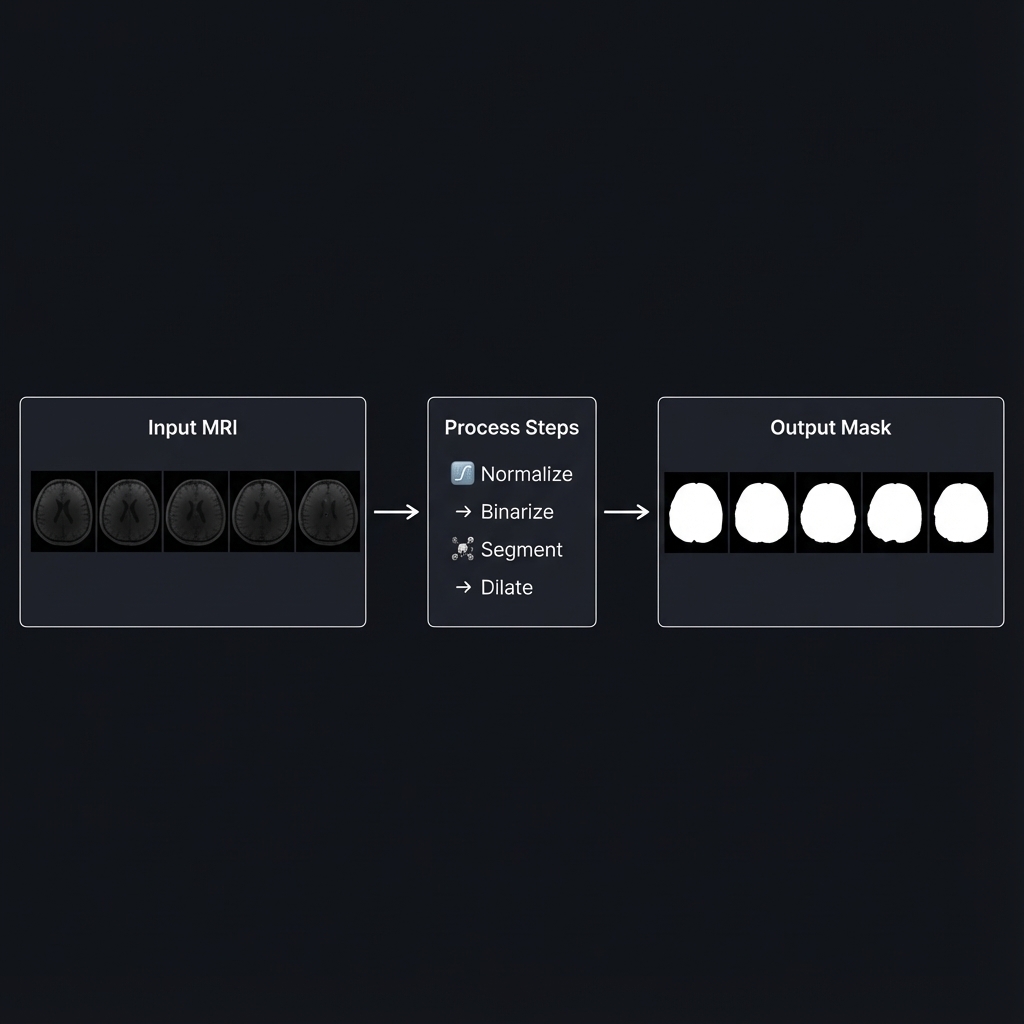
Algorithm Overview

After several iterations (more on that later), I settled on this implementation:

flowchart LR
    subgraph Input
        A[MRI Image<br/>float32]
    end
    
    subgraph Processing
        B[Normalize<br/>0-255] --> C[Otsu<br/>Binarization]
        C --> D[Connected<br/>Components]
        D --> E{Edge<br/>Touching?}
        E -->|Yes| F[Scalp<br/>candidate]
        E -->|No| G[Brain<br/>candidate]
        F --> I[Filter scalp<br/>candidate if present]
        G --> I
        I --> H[Dilation<br/>26px]
        H --> J[Fill<br/>Holes]
    end
    
    subgraph Output
        K[Skull Mask<br/>uint8]
    end
    
    A --> B
    J --> K
    
    style F fill:#d0d4da,color:#333,stroke-dasharray: 5 5
    style G fill:#51cf66,color:#fff
    style K fill:#339af0,color:#fff

The intended rule was: edge-touching bright components can be scalp candidates, while non-edge components can be brain candidates. In the actual 5-slice dataset, the edge-touching bright component counts were [0, 0, 0, 0, 0]. That means the scalp-candidate removal branch existed in the code, but these slices did not exercise it.

The load-bearing path for the reported score was:

1. normalize the image,
2. use Otsu thresholding to find bright tissue,
3. choose the largest internal bright connected component,
4. dilate it by 26px to include the skull boundary,
5. fill internal holes.

The snippets below assume these imports:

import numpy as np
import cv2
from scipy import ndimage

---

Step 1: Normalization

Why Normalize?

cv2.threshold/Otsu work on 8-bit (and 16-bit) single-channel images, so for this pipeline I normalized to 8-bit grayscale. Our raw MRI data ranges from 1.8e-07 to 3.5e-05, and mapping it to a [0, 255] uint8 range keeps the histogram-based threshold well-behaved.

How It Works

def normalize_image(image: np.ndarray) -> np.ndarray:
    img_min = image.min()
    img_max = image.max()
    if img_max == img_min:
        # Flat image: avoid division by zero
        return np.zeros_like(image, dtype=np.uint8)
    img_norm = (image - img_min) / (img_max - img_min)
    img_uint8 = (img_norm * 255).astype(np.uint8)
    return img_uint8

Before: Values in range [1.8e-07, 3.5e-05] After: Values in range [0, 255]

---

Step 2: Otsu Binarization

What Is Binarization?

Binarization converts a grayscale image into a binary image (black and white). Every pixel becomes either 0 (black) or 1 (white) based on a threshold.

The Threshold Selection Problem

If we choose threshold = 100:

• Pixels ≥ 100 → White (1)
• Pixels < 100 → Black (0)

But how do we know 100 is the right value? What if 80 or 120 is better?

Otsu’s Algorithm: Automatic Threshold Selection

Otsu’s method analyzes the histogram and automatically finds the optimal threshold that best separates the two classes (foreground and background).

_, binary = cv2.threshold(img_uint8, 0, 255, cv2.THRESH_BINARY + cv2.THRESH_OTSU)

Across these 5 slices, Otsu landed on threshold = 23 each time (your own data may differ):

Histogram Distribution:

Count
  │
  │  ████                        ████
  │  ████                        ████
  │──────────────────────────────────── Brightness
     0   23                     200
         ↑
    Otsu's optimal split point

Interpretation: Pixels with brightness < 23 are background/skull bone (dark), and pixels ≥ 23 are brain/scalp tissue (bright).

---

Step 3: Connected Components: The Intended Rule

The Intended Rule

After binarization, we have bright regions (tissue) and dark regions (background). The intended connected-component rule was:

Region candidate	Rule
Scalp candidate	A bright component that touches the image border
Brain candidate	A bright component that does not touch the image border

This is a reasonable image-processing heuristic for some cropped slices: outer bright tissue may be connected to the border, while the brain candidate is enclosed inside.

But it did not fire on these 5 slices. After Otsu binarization, the number of edge-touching bright components per slice was:

[0, 0, 0, 0, 0]

So in this dataset, connected components mainly provided a stable largest internal bright component. The scalp-candidate branch was present, but not validated by the sample.

Illustrative Diagram

MRI Image (Binarized):

┌─────────────────────────────────┐
│█████████████████████████████████│← Border-touching bright component
│██                             ██│
│█                               █│← Scalp candidate in the intended rule
│█    ┌───────────────────┐      █│
│█    │                   │      █│
│█    │  Brain candidate  │      █│← No edge contact
│█    │                   │      █│
│█    └───────────────────┘      █│
│██                             ██│
│█████████████████████████████████│
└─────────────────────────────────┘

This diagram explains the intended rule. It is not what happened in the 5 provided slices, where no bright component touched the border.

Implementation

for label in range(1, num_labels):
    component = (labels == label)
    
    touches_edge = any(
        (
            np.any(component[0, :]),    # Top row
            np.any(component[-1, :]),   # Bottom row
            np.any(component[:, 0]),    # Left column
            np.any(component[:, -1]),   # Right column
        )
    )
    
    if touches_edge:
        # Scalp candidate: remove later if present
        edge_labels.add(label)
    else:
        # Brain candidate: keep for largest-component selection
        inner_labels.append(label)

A quick synthetic sanity check confirmed that a border-touching component is labeled as a scalp candidate. That is useful, but it is not the same as validating the path on real MRI slices.

---

Step 4: Morphological Dilation

The Problem

After identifying the brain region, we’re not done yet. The task requires us to include the dark border (skull bone), not just the brain tissue.

The anatomical structure from outside to inside:

[Scalp] → [Skull Bone] → [Brain]
 Bright      Dark        Bright
 Remove      Include     Include

If we only keep the brain region, we miss the skull bone entirely.

The Solution: Dilation

Dilation expands a region by a certain number of pixels in all directions.

Before Dilation:          After Dilation (26px):
┌─────────┐               ┌───────────────┐
│         │               │███████████████│
│  Brain  │      →        │███  Brain  ███│
│         │               │███████████████│
└─────────┘               └───────────────┘

The expanded area covers the Skull Bone region!

Why 26 Pixels?

I tested various dilation sizes:

Dilation Size	IoU	Dice
22	0.9742	0.9869
24	0.9776	0.9887
26	0.9794	0.9896
28	0.9788	0.9893
30	0.9763	0.9880

On these slices, 26 pixels gave the best trade-off: the expanded brain candidate covered the skull boundary, while larger kernels over-expanded past the ground-truth boundary.

The table is the dilation sweep summary. The final all-slice reported score from the full pipeline is IoU 0.9795, Dice 0.9896; the small IoU difference comes from aggregation/rounding details in the sweep versus the final reported average.

---

Step 5: Hole Filling

Why Fill Holes?

After dilation, there might be small holes inside the mask—caused by dark structures within the brain (like ventricles) that were classified as background during binarization.

Before Filling:           After Filling:
┌─────────────┐           ┌─────────────┐
│█████████████│           │█████████████│
│███     █████│           │█████████████│
│███  ○  █████│     →     │█████████████│
│███     █████│           │█████████████│
│█████████████│           │█████████████│
└─────────────┘           └─────────────┘
       ↑
   Internal hole

The skull mask should include the entire interior of the skull, so we fill any internal holes:

skull_mask = ndimage.binary_fill_holes(skull_mask).astype(np.uint8)

---

Understanding the Metrics

IoU (Intersection over Union)

\[\text{IoU} = \frac{|\text{Predicted} \cap \text{Ground Truth}|}{|\text{Predicted} \cup \text{Ground Truth}|}\]

• IoU = 1.0: Perfect overlap
• IoU = 0.0: No overlap at all

Our final all-slice result: IoU = 0.9795 means the intersection is about 97.95% of the union with the ground truth on this tiny set.

Dice Coefficient

\[\text{Dice} = \frac{2 \times |\text{Predicted} \cap \text{Ground Truth}|}{|\text{Predicted}| + |\text{Ground Truth}|}\]

Our result: Dice = 0.9896 is considered excellent in medical image segmentation.

A Note on Validation Limits

These numbers come from just 5 slices, and the dilation size was selected on the same small set. So the result describes how the pipeline fits this provided sample, not how it would generalize.

There is one more important limit: the scalp-candidate removal path was not exercised because the edge-touching bright component count was zero for every slice. Real deployment would need external validation on unseen scans, 3D/volume-level splits (so slices from the same volume don’t leak between tuning and evaluation), and samples where border-touching scalp candidates actually occur. For details on cv2.threshold and Otsu behavior, see the OpenCV imgproc misc docs.

---

The Development Journey

I didn’t arrive at this solution immediately. Here’s my iteration history:

Version	Approach	IoU	Issue
v1	Otsu + Largest Component	0.73	Skull bone not included
v2	Flood Fill from Edges	0.82	Border handling was unstable
v3-v4	Various Thresholds	0.54	Made it worse
v5	Connected Components + Dilation	0.96	Stable brain seed + skull-boundary coverage
v6	Dilation Size Tuning	0.97	Improved
v7	Optimized Dilation (26px)	0.98	Final

The useful shift in v5 was not that the edge branch proved itself on this dataset. It was that connected components gave a stable bright brain candidate, and dilation expanded that candidate far enough to cover the dark skull boundary.

---

Why Not Deep Learning?

Given that this is a segmentation task, you might wonder why I didn’t use U-Net or a similar architecture. Here’s my reasoning:

Criterion	Classical Approach	Deep Learning
Training Data	Not needed	typically many hundreds to thousands of images (rough rule of thumb)
2D Slice Support	✅	✅
External Dependencies	numpy, opencv, scipy	GPU, large frameworks
Interpretability	Each step is clear	Black box
Internal 5-slice IoU	0.98 (5 slices)	Potentially higher with enough data

With only 5 labeled images, deep learning was simply not an option. However, if a substantially larger labeled set (on the order of thousands of images or more) became available, I would consider training a U-Net for potentially even better results.

---

Scaling to 100,000 Images

As part of the project, I also planned for processing 100,000 images within 2 weeks.

Performance Analysis

Metric	Value
Processing time per image	16.6 ms
Images per second	60.2
Time for 100,000 images (single thread)	~28 minutes
Time for 100,000 images (8 cores)	~4 minutes

The classical approach was fast enough for this scale on CPU (single-process vs 8 processes on the (5, 768, 624) slices)—no GPU required!

Batch Processing Script

import numpy as np
from functools import partial
from multiprocessing import Pool

from skull_mask_generator import create_skull_mask


if __name__ == '__main__':
    images = np.load('large_dataset.npy')
    dilation_size = 26
    worker = partial(create_skull_mask, dilation_size=dilation_size)
    
    with Pool(processes=8) as pool:
        masks = pool.map(worker, images)
    
    np.save('output_masks.npy', np.array(masks))

---

Conclusion

Key takeaways:

1. Classical baselines can be useful when labeled data is tiny and the image structure is stable.
2. A high score on 5 tuned slices is not deployment evidence. It is a promising internal fit, not a generalization claim.
3. A code path can exist without being validated. Here, scalp-candidate removal was implemented, but the provided slices never triggered it.

Not every problem needs deep learning, but every strong-looking number needs a careful account of what was actually tested.