MS-CLIP-GAN Architecture: How a CLIP-Guided Multi-Stage GAN Is Wired

Introduction

The previous post in this series fixed the metric: our “FID 0.24” was not a near-perfect generator, but a non-standard 1000-d logit-space FID. Once the measurement was honest, the next question was architectural: what kind of model was actually producing the plateau around FID ~160?

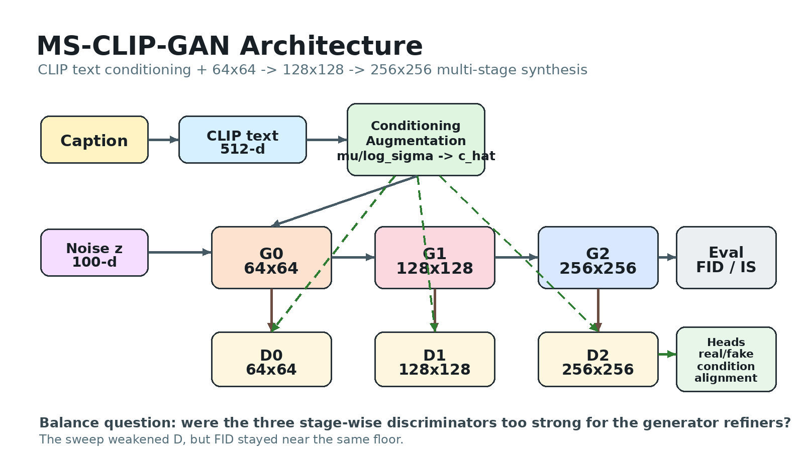
This note is the model map I wanted before interpreting the training curves. MS-CLIP-GAN is not a diffusion model with one denoising U-Net. It is a StackGAN++-style multi-stage GAN with CLIP text conditioning, three generator stages, and three discriminators. That shape matters because the later stability experiment asks a very specific question: was the stage-wise discriminator stack too strong for the generator refiners?

Scope. This is a structural explanation, not a performance claim. The experiment results live in the next post; the metric bug lives in the previous one. Dataset images are licensed, so the figure here is a license-clean architecture diagram rather than generated face samples.

The system in one view: text is embedded by CLIP, compressed through conditioning augmentation, then used by a 64→128→256 generator and three matching discriminators.

The Core Pipeline

At training time, each image-caption pair has already been preprocessed into CLIP features. The text side is a CLIP ViT-B/32 embedding:

caption -> CLIP text encoder -> c_txt (512-d, L2-normalized)

That 512-d vector is not fed directly into every convolutional block. It first passes through a conditioning-augmentation module, inherited conceptually from StackGAN:

c_txt -> linear/ReLU -> mu, log_sigma -> c_hat (128-d)

c_hat is a sampled conditioning vector, regularized with a KL term so the conditioning distribution does not drift arbitrarily. The model then combines c_hat with a 100-d noise vector and generates the image progressively:

Stage	Role	Output
G0	maps text condition + noise into the first image	64×64
G1	refines the previous feature map with the same condition	128×128
G2	refines again into the final image	256×256

That progressive design is the reason the model has a super-resolution flavor: later stages are not starting from scratch; they refine features from earlier stages while seeing the same text condition.

The Discriminator Stack

The adversary is also multi-stage. Each generated image scale has its own discriminator:

Discriminator	Input scale	What it checks
D0	64×64	coarse realism and condition agreement
D1	128×128	mid-level refinement
D2	256×256	final high-resolution realism

Each discriminator compresses its input into a shared feature representation and branches into heads:

• Unconditional real/fake head: is this image real at all?
• Conditional real/fake head: is it real given the text condition?
• Alignment head: does the image feature align with the text feature?

The unconditional head exists in the model, but its loss is opt-in via --use_uncond_loss; the subset experiments discussed in this series enabled it.

The generator also receives auxiliary guidance from a frozen CLIP image encoder at the 256px stage, plus KL and optional perceptual loss. So the training signal is not “just GAN loss”; it is adversarial realism plus semantic alignment and reconstruction-style pressure.

Why the Balance Hypothesis Was Plausible

This architecture makes the discriminator-dominance hypothesis tempting. If one discriminator is too strong, the generator can lose useful gradients. If three discriminators are too strong at three scales, the effect can look even more convincing: D loss falls, G loss rises, and FID gets worse after an early peak.

That is exactly what the baseline curves showed. The model reached its best standard FID around epoch 20, then degraded. On the surface, this looked like a classic “D is winning” story.

The structure makes a clear prediction:

flowchart LR
    A["If the stage-wise D stack is too strong"] --> B["lower D learning rate"]
    A --> C["smooth real labels"]
    A --> D["update D less often"]
    B --> E["FID should improve or stabilize"]
    C --> E
    D --> E

That prediction is what the next post tested. The result was negative: weakening D did not robustly improve FID, and the model stayed around the same ~160 floor.

Compared With RTMDet

This is where the RTMDet paper-review style is useful. RTMDet and MS-CLIP-GAN are different kinds of models, but the way to read them is similar: understand the architecture first, then ask whether the experiment actually tests the right part of that architecture.

Aspect	RTMDet	MS-CLIP-GAN
Task	object detection	text-to-image generation
Core shape	backbone → neck → detection head	CLIP condition → staged generator → staged discriminators
Multi-scale role	feature pyramid for boxes at different strides	image synthesis/refinement at 64/128/256
Main metric	COCO-style mAP	standard 2048-d FID / IS
Failure mode studied	false positives despite high mAP	FID plateau despite GAN-balance tuning
Lesson	architecture is strong, but evaluation/data can still hide deployment failures	architecture runs, but the bottleneck is likely data/objective/model capacity rather than D-balance

RTMDet is a mature detector whose paper carefully ablates backbone, neck, head, label assignment, and training schedule. MS-CLIP-GAN is a project implementation that combines StackGAN++-style staging, CLIP conditioning, and auxiliary losses. So the standard of evidence is different. RTMDet’s architecture is the thing the paper validates; MS-CLIP-GAN’s architecture is the thing we must audit before trusting the experiment.

The common lesson is the same one this blog keeps coming back to: a model diagram is not decoration. It tells you what hypotheses are even meaningful. In RTMDet, the natural questions are about feature pyramids, assignment, and dataset leakage. In MS-CLIP-GAN, the natural question was whether the multi-scale discriminator stack was overpowering the generator.

What This Architecture Does Not Prove

The diagram explains the training dynamics, but it does not rescue the results. The subset experiment still plateaued around FID ~160, and the best checkpoint still came from the baseline epoch-20 run.

The main limitations follow directly from the structure:

• The text condition is only a CLIP embedding, not a token-level cross-attention mechanism.
• The 256px stage is asked to learn real high-resolution detail from a small subset.
• Three discriminators provide strong feedback, but also make optimization noisy.
• CLIP guidance helps semantic alignment, but it is not a full image-quality objective.

So future gains probably require more than tuning d_lr or n_critic: larger data, stronger conditioning, a better objective mix, or a more modern generator family.

Resources

• Previous in this series — the metric fix that made the experiments meaningful: “Your FID of 0.24 Isn’t Near-Perfect”
• Next in this series — the stability sweep that tested the D-dominance hypothesis: “Killing a Hypothesis Cheaply”
• Architecture relatives — StackGAN++ (arXiv:1710.10916), LAFITE (arXiv:2111.13792), and the RTMDet review’s architecture-first framing: “RTMDet: An Empirical Study of Designing Real-Time Object Detectors”