[Paper Review] Deep Unsupervised Learning using Nonequilibrium Thermodynamics

Note: This is a review of “Deep Unsupervised Learning using Nonequilibrium Thermodynamics” (Sohl-Dickstein, Weiss, Maheswaranathan & Ganguli; ICML 2015, PMLR v37 pp. 2256-2265; arXiv:1503.03585, doi:10.48550/arXiv.1503.03585).

Code: Sohl-Dickstein/Diffusion-Probabilistic-Models (the original Theano/Blocks reference implementation).

For a thorough Korean walkthrough, see 최민서 (Choi Min-seo)’s “Deep Unsupervised Learning using Nonequilibrium Thermodynamics” 논문 리뷰 (OUTTA AI Tech Blog, 2025-01-03). This post doesn’t retread that ground – see below.

All figures here are original – the paper’s arXiv license (nonexclusive-distrib/1.0) is not Creative Commons, and one figure is separately licensed from a third party, so nothing is reproduced from the PDF. Tables and equations are retyped from the source (facts/equations aren’t copyrightable expression).

Why I Read This Paper

I came to this paper backwards, via an audit of a broken PyTorch reimplementation of it whose MNIST path had quietly dropped the forward posterior the paper’s entire training objective is built from. Fixing that meant reading the 2015 paper closely enough to know exactly which quantity was missing, and why the training sum starts at $t=2$, not $t=1$ – a different kind of reading than a first-pass summary turns up.

최민서’s OUTTA review linked above already covers the abstract, algorithm, and experiments end to end, derivations included, so I’m not re-deriving that. This review is written from an implementer’s seat instead: an architectural detail that’s a common source of bugs, a footnote that quietly kills half of DDPM’s design space, a table cell that disagrees with the text next to it, and a sentence in Appendix C that is classifier guidance five to six years before anyone called it that.

---

Introduction

The paper opens from an old tension in generative modeling: tractability versus flexibility. A model flexible enough to fit any data distribution usually has an intractable normalizing constant $Z$, so $p(x) = \phi(x)/Z$ can’t be evaluated, sampled cheaply, or fit by maximum likelihood without an approximation. The introduction surveys the existing menu – mean field, variational Bayes, contrastive divergence, minimum probability flow, score matching, pseudolikelihood, loopy belief propagation, non-parametric methods – then proposes a different escape hatch.

The idea in one sentence: build a Markov chain that slowly destroys structure in the data with a simple diffusion kernel until the data distribution has become a known one (isotropic Gaussian, or independent Bernoulli), then learn to run that chain backwards. Because the forward chain is restricted to a simple, tractable functional form, the reverse chain can share that same form – so the generative model becomes, layer by layer, a sequence of regressions.

The paper’s stated payoff (§1.1): extreme flexibility, exact sampling (no MCMC, no rejection), easy multiplication with other distributions (posteriors like inpainting fall out almost free), and cheap log-likelihood evaluation. Against the contemporaneous VAE line (§1.2) it claims five distinguishing features: that same multiplication property; a physics/quasi-static/AIS framing rather than variational Bayes; no separate inference network to train, since the forward process is the inference process; thousands of layers instead of a handful; and analytic entropy-production bounds per step.

There is no boxed Algorithm 1 anywhere – training and sampling are described entirely in prose, unlike DDPM’s two algorithm boxes.

Context / Related Work

The paper positions itself against three neighborhoods: the classical intractability toolbox above (MCMC-adjacent and pseudo-likelihood methods approximating the partition function rather than sidestepping it); wake-sleep and the VAE family (Kingma & Welling; Gregor, Danihelka, Mnih, Blundell & Wierstra; Rezende, Mohamed & Wierstra) – the family the Introduction’s “no inference network” and physics-framing claims (quasi-static processes, Jarzynski’s equality, AIS) are directed against; and a physics lineage (Burda et al.’s reverse-AIS estimator, Langevin dynamics, the Fokker-Planck equation, and the Kolmogorov forward/backward equations, Feller 1949, that justify why a reverse chain can share the forward chain’s form in the small-step limit).

This is not a review of DDPM, which postdates this paper by five years and is never mentioned in it – but because much of what follows will sound familiar to DDPM readers, I flag the connection at each relevant point.

---

Method

1. Forward and reverse trajectories, in two flavors

Superscripts index diffusion timesteps: $x^{(0)}$ is a data point, $x^{(T)}$ is pure noise, and $q$/$p$ denote the forward and reverse processes. The forward step (Eq. 2) applies a fixed kernel $T_\pi(x^{(t)} \mid x^{(t-1)}; \beta_t)$ at rate $\beta_t$, chosen so the kernel’s own invariant distribution $\pi$ (Eq. 1) is the chain’s endpoint. The paper works out two instantiations, side by side in Table App.1:

	Gaussian	Binomial
Base distribution $\pi(x^{(T)})$	$\mathcal{N}(x^{(T)}; 0, I)$	$B(x^{(T)}; 0.5)$
Forward kernel $q(x^{(t)}\mid x^{(t-1)})$	$\mathcal{N}!\left(x^{(t)}; x^{(t-1)}\sqrt{1-\beta_t},\, I\beta_t\right)$	$B!\left(x^{(t)}; x^{(t-1)}(1-\beta_t) + 0.5\beta_t\right)$
Reverse kernel $p(x^{(t-1)}\mid x^{(t)})$	$\mathcal{N}!\left(x^{(t-1)}; f_\mu(x^{(t)}, t),\, f_\Sigma(x^{(t)}, t)\right)$	$B!\left(x^{(t-1)}; f_b(x^{(t)}, t)\right)$
Training targets	$f_\mu,\, f_\Sigma,\,$ and $\beta_{1\ldots T}$	$f_b$ only

Table App.1 (partial, retyped): the paper’s own cheat-sheet, between Appendices B and C. Row order and cell content are exact; I’ve kept only the rows relevant here.

The Gaussian forward kernel here is byte-for-byte what DDPM later calls its forward process. What is not in this paper is the closed-form marginal $q(x^{(t)}\mid x^{(0)})$ DDPM writes explicitly in terms of $\bar\alpha_t = \prod_{s\le t}(1-\beta_s)$ – there is no $\bar\alpha$ notation anywhere here. The paper only asserts that the relevant entropies and KLs “can be analytically computed given $x^{(0)}$ and $x^{(t)}$” (end of Appendix B.4); DDPM’s contribution is making that closed form explicit and reparameterizing on top of it.

Look at the Training targets row: for the Gaussian case, the schedule $\beta_{1\ldots T}$ is itself a training target – learned, not fixed (Section 3 below, the row this paper most directly disagrees with itself over).

For the binomial case $\beta$ cannot be learned this way at all: “the discrete state space makes gradient ascent with frozen noise impossible” (§2.4.1), so it is set analytically to erase a constant fraction $1/T$ of signal per step, $\beta_t = (T-t+1)^{-1}$.

Sampling (§2.2, Eq. 5) draws $x^{(T)} \sim \pi$ and runs the learned reverse kernel down to $x^{(0)}$ – $T-1$ sequential network evaluations plus the fixed final step (Eq. 44, Section 2 below), no shortcuts. The paper is explicit these are true samples, not the final Gaussian’s posterior mean – a distinction its Figure App.1 caption calls out for MNIST.

2. From an intractable integral to a trainable bound

The model likelihood (Eq. 6) is $p(x^{(0)}) = \int dx^{(1\ldots T)}\, p(x^{(0\ldots T)})$, an integral the paper calls naively intractable. The move (Eqs. 7-9) is the standard AIS trick: multiply and divide by the forward conditional $q(x^{(1\ldots T)}\mid x^{(0)})$, turning the integral into an importance-weighted expectation over forward-process samples,

\[p(x^{(0)}) = \int dx^{(1\ldots T)}\; q(x^{(1\ldots T)}\mid x^{(0)}) \cdot p(x^{(T)}) \prod_{t=1}^{T} \frac{p(x^{(t-1)}\mid x^{(t)})}{q(x^{(t)}\mid x^{(t-1)})}. \tag{9}\]

The training objective is the expected log-likelihood over the data distribution,

\[L = \int dx^{(0)}\, q(x^{(0)}) \log p(x^{(0)}), \tag{10}\]

with Eq. 9 substituted inside the log (Eq. 11, not reproduced here). Jensen’s inequality then moves the log inside the expectation over the whole trajectory rather than just $x^{(0)}$, which can only decrease the bound:

\[L \;\ge\; \int dx^{(0\ldots T)}\, q(x^{(0\ldots T)}) \, \log\!\left[\, p(x^{(T)}) \prod_{t=1}^{T} \frac{p(x^{(t-1)}\mid x^{(t)})}{q(x^{(t)}\mid x^{(t-1)})} \,\right] \;=:\; K, \tag{12,13}\]

so $L \ge K$, and Appendix B reduces $K$ (via the entropy identities in B.1, the edge-effect trick in B.2 below, and the Bayes-rule swap in B.3-B.4) to the form the paper actually trains against:

\[K = -\sum_{t=2}^{T} \int dx^{(0)}\,dx^{(t)}\; q\!\left(x^{(0)}, x^{(t)}\right) \, D_{\mathrm{KL}}\!\Big(\, q(x^{(t-1)}\mid x^{(t)}, x^{(0)}) \;\Big\|\; p(x^{(t-1)}\mid x^{(t)}) \,\Big) \; + \; H_q\!\left(X^{(T)} \mid X^{(0)}\right) - H_q\!\left(X^{(1)} \mid X^{(0)}\right) - H_p\!\left(X^{(T)}\right). \tag{14}\]

That KL term is the whole paper: it matches the learned reverse kernel $p(x^{(t-1)}\mid x^{(t)})$ to the forward posterior conditioned on the clean data, $q(x^{(t-1)}\mid x^{(t)}, x^{(0)})$ – exactly the object DDPM calls $L_{t-1}$ five years later. DDPM’s addition is the closed form of that posterior (via $\bar\alpha_t$) and an $\epsilon$-reparameterization on top, not the objective itself.

First, why the sum starts at $t=2$, not $t=1$: Appendix B.2 handles the $t=0$ edge case by defining the final reverse step to equal the forward step run backwards,

\[p(x^{(0)} \mid x^{(1)}) \;=\; q(x^{(1)} \mid x^{(0)}) \, \frac{\pi(x^{(0)})}{\pi(x^{(1)})} \;=\; T_\pi\!\left(x^{(0)} \mid x^{(1)}; \beta_1\right), \tag{44}\]

removing that step from the sum entirely – it’s a fixed identity, not learned – which is why Eq. 14’s KL sum runs $t = 2 \ldots T$. Second, the bound is tight ($L = K$, equality in Eq. 13) only in the quasi-static limit of infinitesimal $\beta$, where forward and reverse trajectory distributions coincide. Every reported number is a lower bound, and the smaller $\beta$ can be made (at the cost of a longer trajectory), the tighter it gets.

3. Setting the diffusion rate $\beta_t$ – the single most under-quoted footnote in this paper

Table App.1’s “Training targets” row says the Gaussian case learns $\beta_{1\ldots T}$. Section 2.4.1’s text is more careful: “we learn the forward diffusion schedule $\beta_{2\ldots T}$ by gradient ascent on $K$. The variance $\beta_1$ of the first step is fixed to a small constant to prevent overfitting.” That’s already a small inconsistency – the table’s blanket $\beta_{1\ldots T}$ vs. the text’s $\beta_{2\ldots T}$ with $\beta_1$ held out (the first of three, cataloged below).

The sentence that matters most is a footnote on the word “learn,” easy to skip past:

“Recent experiments suggest that it is just as effective to instead use the same fixed $\beta_t$ schedule as for binomial diffusion.”

The paper spends a page justifying gradient ascent on $\beta$ with the reparameterization trick and “frozen noise,” then, in a footnote, says it probably didn’t need to. This is the direct textual ancestor of DDPM’s decision, five years later, to fix $\beta_t$ to a hand-set schedule and drop it from the learned parameters entirely – DDPM states that design choice without citing this footnote, but the idea is here first.

The Gaussian case has no closed-form schedule of its own anywhere in this paper – Table App.1’s “Training targets” row, and the more careful text above it, both say $\beta_{2\ldots T}$ is learned for Gaussian diffusion, not given analytically. What footnote 2 licenses is reusing the schedule the paper derives for the other branch: the binomial case’s closed form from Section 1 above, $\beta_t = (T-t+1)^{-1}$ (§2.4.1, forced there by the discrete-state-space constraint already quoted). That formula is never derived for Gaussian diffusion in this paper; footnote 2 is the entire justification for carrying it over. DDPM’s schedule is linear from $10^{-4}$ to $0.02$. Both are “fixed” in the sense the footnote endorses, but they look nothing alike – and, as the next two paragraphs show, the binomial formula’s own closed form and the paper’s own released code for it don’t even agree with each other:

import numpy as np


def sohl_dickstein_2015_paper_schedule(T: int) -> np.ndarray:
    # beta_t = (T-t+1)^-1 -- binomial formula (Sec. 2.4.1), via footnote 2
    t = np.arange(1, T + 1)
    return 1.0 / (T - t + 1)
# end def


def sohl_dickstein_2015_released_code_schedule(T: int) -> np.ndarray:
    # released Theano code (model.py): (T-t+2)^-1, not (T-t+1)^-1
    return 1.0 / np.linspace(T, 2, T)
# end def


def ddpm_2020_schedule(T: int, beta_start: float = 1e-4, beta_end: float = 0.02) -> np.ndarray:
    return np.linspace(beta_start, beta_end, T)  # Ho, Jain & Abbeel 2020, Sec. 4
# end def


def alpha_bar(beta_t: np.ndarray) -> np.ndarray:
    return np.cumprod(1.0 - beta_t)  # prod_{s=1..t}(1 - beta_s)
# end def


T = 1000
beta_paper = sohl_dickstein_2015_paper_schedule(T)
beta_code = sohl_dickstein_2015_released_code_schedule(T)
beta_ddpm = ddpm_2020_schedule(T)
print(f"paper formula: beta_1={beta_paper[0]:.4f} beta_T={beta_paper[-1]:.2f} alpha_bar_T={alpha_bar(beta_paper)[-1]:.2e}")
print(f"released code: beta_1={beta_code[0]:.4f} beta_T={beta_code[-1]:.2f} alpha_bar_T={alpha_bar(beta_code)[-1]:.2e}")
print(f"DDPM:          beta_1={beta_ddpm[0]:.4f} beta_T={beta_ddpm[-1]:.2f} alpha_bar_T={alpha_bar(beta_ddpm)[-1]:.2e}")
# paper formula: beta_1=0.0010 beta_T=1.00 alpha_bar_T=0.00e+00
# released code: beta_1=0.0010 beta_T=0.50 alpha_bar_T=9.94e-04
# DDPM:          beta_1=0.0001 beta_T=0.02 alpha_bar_T=4.04e-05

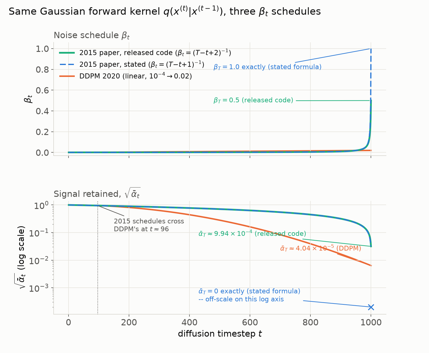
Both closed forms are exact, and they disagree about where the trajectory ends. The paper’s stated formula, $\beta_t = (T-t+1)^{-1}$, telescopes to $\bar\alpha_t = 1 - t/T$ exactly – at $t=500$, $T=1000$, that’s $\bar\alpha_t = 1 - 500/1000 = 0.500000$ exactly – so $\bar\alpha_T = 0$ exactly at $t=T$: the schedule really does erase a constant fraction $1/T$ of the original signal every step, all the way to nothing, exactly as its own “constant fraction of signal per step” framing (Section 1 above) claims.

The paper’s own released reference implementation computes something else: beta_baseline = 1./np.linspace(trajectory_length, 2., trajectory_length), i.e. $\beta_t = (T-t+2)^{-1}$, not $(T-t+1)^{-1}$ – a one-index shift easy to miss by eye. The same telescoping argument gives it a clean closed form too, $\bar\alpha_t = (T-t+1)/(T+1)$, so $\bar\alpha_T = 1/(T+1) \approx 9.99\times10^{-4}$, not zero. Actually executing 1./np.linspace(T, 2, T) for $T=1000$ (the print statements above) lands a hair below that, $\bar\alpha_T \approx 9.94\times10^{-4}$, because NumPy’s linspace step between $T$ and $2$ is $(T-2)/(T-1) \approx 0.999$, not exactly $1$ – close enough at $T=1000$ that the two only disagree in the third significant figure.

So the paper’s stated formula and its own released code disagree about the terminal step: $\bar\alpha_T = 0$ exactly by the text, $\bar\alpha_T \approx 9.94\times10^{-4}$ by the code the same authors shipped – a fourth internal inconsistency, different in kind from the three cataloged at the end of this section: those are text disagreeing with text, this is text disagreeing with code. It matters more than the other three for anyone reimplementing this paper: the companion audit post’s reimplementation traces back, through a chain of refactors, to this exact released repository, and inherits 1./np.linspace(T, 2, T) – the released-code variant, not the paper’s own stated formula.

Same Gaussian forward kernel, three $\beta_t$ schedules (original chart, computed and rendered for this post). The paper’s stated formula and its own released code track each other almost exactly until the last few steps ($\beta_1{=}0.001$ for both), since they differ by only one index; both cross above DDPM’s linear schedule at $t\approx96$ – about 9.6% into the trajectory – and hold more signal than DDPM for the rest of the run. Only in the final step do the two 2015 curves split from each other: the stated formula’s $\bar\alpha_t$ crashes to exactly $0$ (off-scale on this log axis, marked with an $\times$ at the floor), while the released code’s $\bar\alpha_T \approx 9.94\times10^{-4}$ – both still above DDPM’s $\bar\alpha_T \approx 4.04\times10^{-5}$.

Worth flagging: the companion audit post reports a fourth number easy to conflate with these, $\bar\alpha_T \approx 5.5\times10^{-14}$ with 79% of trained timesteps at $\sqrt{\bar\alpha_t} < 0.1$ – belonging to none of the three schedules above. It’s what the audited repo’s pre-fix code actually ran, beta = linspace(0.01, 0.05, 1000), steeper at both ends than DDPM’s own schedule and unrelated to either variant of this paper’s analytic form.

4. The architecture: two pathways, and time is not an input

Appendix D.2.1 describes one shared architecture for all four image datasets (MNIST, CIFAR-10, dead leaves, bark), built from two parallel pathways feeding a shared readout:

flowchart LR
    IN["Input x^(t)"] --> DP["Dense pathway<br/>(full image vector -> tanh)"]
    IN --> MS["Multi-scale conv pathway<br/>(pool to scales -> conv -> upsample+sum -> soft-relu)"]
    DP --> C1["1x1 conv<br/>(per-pixel feature vector -> tanh)"]
    MS --> C1
    C1 --> Y["Readout y_i in R^2J<br/>split y^mu, y^Sigma"]
    Y --> TB["Temporal bump basis g_j(t)<br/>softmax-normalized Gaussian (Eq. 63)"]
    TB --> ZM["z^mu_i, z^Sigma_i (Eq. 62)"]
    ZM --> MEAN["Mean image mu_i (Eq. 65)<br/>perturbation around forward kernel"]
    ZM --> COV["Covariance image Sigma_ii (Eq. 64)<br/>diagonal"]

Redrawn from the paper’s Appendix D.2.1 description of Figure D.1 (original diagram; not reproduced here). The paper states the pathway rule for only two of its four datasets: for CIFAR-10, the dense pathway ran in parallel with the multi-scale convolutional pathway; for MNIST, it was used to the exclusion of the convolutional pathway (so the published MNIST model is effectively a dense/MLP model). Bark and dead leaves aren’t stated.

Two things matter for implementation. First, §2.2 flatly states “For all results in this paper, multi-layer perceptrons are used to define these functions” – directly contradicting the convolutional, multi-scale architecture D.2.1 spends a full page describing (internal inconsistency #2 of three, cataloged below); D.2.1 is the specific, correct source.

Second, the detail most likely to trip up a reimplementation: the network itself is not a function of $t$. At each timestep the conv/dense stack runs on $x^{(t)}$ alone, emitting a per-pixel coefficient vector $y_i \in \mathbb{R}^{2J}$ – no timestep embedding enters the network. Time enters only at readout, as a fixed, softmax-normalized Gaussian “bump” basis:

\[z^{\mu}_i = \sum_{j=1}^{J} y^{\mu}_{ij}\, g_j(t), \qquad g_j(t) = \frac{\exp\!\big(-(t-\tau_j)^2 / 2w^2\big)}{\sum_{k=1}^{J} \exp\!\big(-(t-\tau_k)^2 / 2w^2\big)}, \tag{62,63}\]

with bump centers $\tau_j$ spread across $(0,T)$, spaced $w$ apart – $w$ is the spacing between adjacent bump centers, not a shared width parameter, despite also setting the Gaussian’s variance in Eq. 63’s denominator. Get that wrong and bumps end up misspaced or with the wrong width. This is a learned-coefficient, fixed-basis interpolation across timesteps – the opposite of DDPM’s approach, which shares one network across all $t$ and injects a sinusoidal position embedding into every residual block. Neither $J$ nor $w$ is ever given a numeric value in the paper – treat both as unspecified.

The mean and diagonal covariance outputs are parameterized as small perturbations around the forward kernel itself, $\Sigma_{ii} = \sigma\big(z^\Sigma_i + \sigma^{-1}(\beta_t)\big)$ and $\mu_i = (x_i - z^\mu_i)(1-\Sigma_{ii}) + z^\mu_i$ (Eqs. 64-65) – a network outputting all zeros recovers the forward kernel’s variance exactly and its mean to first order in $\beta_t$ ($x_i(1-\beta_t)$ vs. the forward kernel’s $x_i\sqrt{1-\beta_t}$; the two agree as $\beta_t \to 0$ but diverge at the large $\beta_t$ this schedule reaches near $t=T$).

5. Two ideas that resurfaced later, under different names

Both rediscovered under new names well after 2015, and this paper rarely gets cited for either.

The entropy bound. Section 2.6 (Eq. 24) gives an analytic two-sided bound on each reverse step’s conditional entropy, purely in terms of the forward process:

\[H_q(X^{(t)}\mid X^{(t-1)}) + H_q(X^{(t-1)}\mid X^{(0)}) - H_q(X^{(t)}\mid X^{(0)}) \;\le\; H_q(X^{(t-1)}\mid X^{(t)}) \;\le\; H_q(X^{(t)}\mid X^{(t-1)}). \tag{24}\]

DDPM cites exactly this result to justify its two fixed choices of reverse variance, $\sigma_t^2 \in {\beta_t, \tilde\beta_t}$, as “the two extreme choices corresponding to upper and lower bounds on reverse process entropy.”

Classifier guidance, six years early. Appendix C derives sampling from a perturbed model $\tilde p(x^{(0)}) \propto p(x^{(0)})\, r(x^{(0)})$ – multiplying the learned distribution by another function $r$, e.g. a delta function on observed pixels for inpainting, or a likelihood term for denoising. Table App.1’s perturbed Gaussian reverse kernel, derived at Eq. 61, is:

\[\tilde p(x^{(t-1)}\mid x^{(t)}) = \mathcal{N}\!\Big(x^{(t-1)};\; f_\mu(x^{(t)},t) + f_\Sigma(x^{(t)},t)\, \nabla \log r(x^{(t-1)})\Big|_{x^{(t-1)} = f_\mu(x^{(t)},t)},\;\; f_\Sigma(x^{(t)},t)\Big).\]

Strip the notation and this says: shift the reverse-step mean by the covariance times the gradient of $\log r$. That is, structurally, classifier guidance – the technique commonly cited to Dhariwal & Nichol’s 2021 “Diffusion Models Beat GANs,” where $r$ is a classifier’s class-conditional likelihood and the same $\Sigma \cdot \nabla \log r$ shift steers sampling toward a target class. This paper derives the general mechanism in 2015, six years before the name existed, for multiplying a diffusion model by any smooth function – inpainting and denoising are just the two instances its experiments happen to use.

Experiments / Results

Table 1: the log-likelihood lower bound, six datasets

Dataset	K	K − L_null
Swiss Roll	2.35 bits	6.45 bits
Binary Heartbeat	−2.414 bits/seq.	12.024 bits/seq.
Bark	−0.55 bits/pixel	1.5 bits/pixel
Dead Leaves	1.489 bits/pixel	3.536 bits/pixel
CIFAR-10	5.4 ± 0.2 bits/pixel	11.5 ± 0.2 bits/pixel
MNIST	see Table 2	see Table 2

Table 1 (numbers from the paper, Table 1; see Eq. 12 in the paper for the definition of $K$). $L{\mathrm{null}}$ is the log-likelihood of the base distribution $\pi(x^{(0)})$ scored on the same data – the right column is the improvement over that null model. All datasets except Binary Heartbeat were rescaled to unit variance before computing log-likelihood, and CIFAR-10 is the only row carrying an error bar (from the released reference implementation’s standard-error report). CIFAR-10 is bold as the highest $K$ in the table._

Two caveats. These are differential-entropy-style bounds on unit-variance-rescaled continuous data, so they are not on the same scale as modern bits/dim figures on 8-bit discrete pixels (DDPM’s $\le 3.75$ bits/dim on CIFAR-10) – don’t compare directly.

Footnote 3, on the CIFAR-10 row: “An earlier version of this paper reported higher log likelihood bounds on CIFAR-10. These were the result of the model learning the 8-bit quantization of pixel values… The log likelihood bounds reported here are instead for data that has been pre-processed by adding uniform noise to remove pixel quantization.” The superseded numbers – 11.895 / 18.037 bits/pixel – survive only as a commented-out LaTeX line; they were the model exploiting a measurement artifact, caught and retracted before this version. Do not cite 11.895/18.037 as a result of this paper – 5.4 ± 0.2 above is the corrected, published figure.

Table 2: MNIST and dead leaves against other models

Model	Log Likelihood
Dead Leaves
MCGSM	1.244 bits/pixel
Diffusion	1.489 bits/pixel
MNIST
Stacked CAE	174 ± 2.3 bits
DBN	199 ± 2.9 bits
Deep GSN	309 ± 1.6 bits
Diffusion	317 ± 2.7 bits
Adversarial net	325 ± 2.9 bits
Perfect model	349 ± 3.3 bits

Table 2 (numbers from the paper, Table 2). Dead leaves uses identical train/test data to Theis et al. 2012, so the MCGSM row is a like-for-like comparison and the paper’s clearest state-of-the-art claim (bold: 1.489 vs. 1.244 bits/pixel). MNIST numbers are Parzen-window estimates, computed with the code released alongside Goodfellow et al. 2014’s GAN paper, converted to bits.

The MNIST block deserves a second look: the diffusion model is not the best row, beating Deep GSN but sitting below “Adversarial net” (317 vs. 325 bits). More interesting is the row below that: “Perfect model,” 349 ± 3.3 bits, is not a model at all – it’s the same Parzen-window estimator applied directly to samples from the training data itself, so it measures the ceiling of the evaluation metric, not of any generative model. The paper reports this without comment, but it’s a tacit admission that Parzen-window log-likelihood is a weak, noisy metric: even ground-truth data doesn’t score much above a working model (349 vs. 317) – the metric has limited resolving power at this scale.

Three places where the paper disagrees with itself

1. The $\beta$-learning target (Method §3, above). Table App.1 lists the Gaussian training target as $\beta_{1\ldots T}$; §2.4.1’s prose is more specific and says only $\beta_{2\ldots T}$ is learned, with $\beta_1$ fixed “to prevent overfitting.” The prose is the more authoritative statement.
2. “Multi-layer perceptrons,” except when they’re convolutions (Method §4, above). §2.2 says all reported results use MLPs to define $f_\mu$/$f_\Sigma$/$f_b$; Appendix D.2.1 describes a genuinely convolutional, multi-scale architecture. D.2.1 wins – the specific, detailed description beats the paper’s own loose summary.
3. The binomial base rate: 0.5 in the table, 0.2 in the appendix – and the arithmetic proves which one actually ran. Table App.1 states the binomial base distribution is $B(x^{(T)}; 0.5)$. Appendix D.1.2, describing the binary-heartbeat experiment, initializes at $p(x_i^{(T)}=1) = 0.2$, “the same mean activity as the data.” Both can’t be what ran – Table 1’s own numbers settle it. Table 1 reports, for Binary Heartbeat, $K = -2.414$ and $K - L_{\mathrm{null}} = 12.024$ bits/sequence, so $L_{\mathrm{null}} = -14.438$ bits/sequence. The sequences are 20 bits long, and $H(0.2) = -0.2\log_2 0.2 - 0.8\log_2 0.8 = 0.72193$ bits, so twenty independent bits at that rate cost

\[20 \times H(0.2) = 20 \times 0.72193 = 14.4386 \text{ bits} \;\approx\; -L_{\mathrm{null}} = 14.438.\]

An exact match to four significant figures. Twenty independent Bernoulli($0.5$) bits would instead cost exactly 20 bits, not 14.4386 – the arithmetic rules that out. 0.2 is what actually ran; Table App.1’s “0.5” is the error. (The paper’s own prose description of this initialization, “with identical mean activation rate to the training data,” is present in the LaTeX source but commented out of the published PDF – the appendix’s 0.2 is the only place the correct value survives in print.)

The two conditional demonstrations

The paper exercises the Eq. 61 machinery twice: on CIFAR-10 (Figure 3), holdout images corrupted with Gaussian noise at SNR = 1 are run through the perturbed reverse chain to produce a sample from the posterior over denoised images – an actual draw, not a MAP estimate or conditional mean; and on bark textures (Figure 5, Lazebnik et al. 2005), a 100×100 center region replaced with isotropic Gaussian noise is inpainted the same way, $r(x^{(0)})$ a delta function on known pixels and a constant on missing ones (the exact-multiplication case §2.5.3 covers cleanly). Neither figure is reproduced here for the licensing reasons noted at the top.

---

Conclusion & Insight

This paper reads, eleven years later, less like “one interesting idea” and more like a blueprint built out piece by piece by other people – the forward/reverse Gaussian process, the per-step KL objective, the entropy bounds, and the guidance mechanism are all here in 2015 form, years before each became a headline result under someone else’s name.

Strengths

• The core argument is genuinely elegant. Restricting the forward process to a simple form, and arguing the reverse can share that form (Feller’s small-step result), sidesteps the “train a good inference network” problem VAEs wrestle with – by construction, not regularization.
• The math is more complete than it gets credit for. The variational bound (Eqs. 10-14), the entropy bounds (Eq. 24), and the guidance mechanism (Eq. 61) are all derived rigorously in the appendices, not asserted.
• It’s honest about being a lower bound. Every reported number is framed as $K \le L$, tight only in the quasi-static limit.
• The retraction (footnote 3) is a good look, not a bad one. Catching and correcting a measurement artifact before publication, with a footnote explaining exactly what happened, is rigor a lot of papers skip.

Limitations

• No dedicated limitations section, no algorithm box. Every limitation here was assembled from scattered caveats, not a place the authors put together themselves.
• Cost scales linearly with trajectory length, and the paper’s own flexibility argument (smaller $\beta$ needs a longer trajectory) works directly against sampling speed – 999 sequential network evaluations for the image experiments ($T=1000$ for MNIST, CIFAR-10, and dead leaves; $T=500$ for bark), no shortcut available (this predates DDIM-style step-skipping by five years).
• The MNIST evaluation metric is weak, and the paper’s own “Perfect model” row proves it: ground-truth data scores only marginally above a working model.
• Key hyperparameters are simply missing. $J$ and $w$ of the bump basis are never given numeric values; nor are parameter counts, learning rates, batch sizes, or wall-clock time for any image experiment.
• Internal inconsistencies, cataloged above, mean the paper can’t quite be read as an unambiguous spec – Table App.1 and the prose disagree twice, and one number (0.2 vs. 0.5) is only resolvable by doing the arithmetic yourself.

Open Questions / My Take

The implementer’s-seat framing of this review comes from the companion audit: its reimplementation still doesn’t produce recognizable MNIST digits from pure noise, even after fixing the missing-forward-posterior defect this paper’s Eq. 14 is built around, though the denoiser itself demonstrably works (see that post for the full picture). That gap isn’t evidence against anything in this paper – rereading it closely mainly surfaced more places a from-scratch implementation can silently diverge than expected: the bump-basis time-conditioning, the exact $\beta$ schedule, the two-pathway architecture, the $\beta_1$ edge case.

What I’d want to see next: a from-scratch, paper-faithful (not DDPM-flavored) reimplementation reporting the same unnormalized, unit-variance-rescaled bits/pixel numbers this paper reports, so the 5.4 ± 0.2 CIFAR-10 and 1.489 dead-leaves figures above are checkable against a modern run rather than only against the paper’s own 2015-era Theano code. I’m not aware of anyone who has done that.

Resources

• Companion post – the implementer’s audit: what a broken reimplementation of this exact paper looked like from the inside
• Paper – Sohl-Dickstein, Weiss, Maheswaranathan & Ganguli, Deep Unsupervised Learning using Nonequilibrium Thermodynamics, ICML 2015 (arXiv:1503.03585)
• Reference implementation – Sohl-Dickstein/Diffusion-Probabilistic-Models (Theano/Blocks)
• Korean review – 최민서, “Deep Unsupervised Learning using Nonequilibrium Thermodynamics” 논문 리뷰, OUTTA AI Tech Blog, 2025-01-03
• Successor – Ho, Jain & Abbeel, Denoising Diffusion Probabilistic Models, NeurIPS 2020 (arXiv:2006.11239) – keeps this paper’s forward kernel and variational bound; fixes $\beta$ (footnote 2 said that was fine); replaces the learned reverse variance with two fixed choices justified by this paper’s Eq. 24; reparameterizes the mean as noise prediction
• Related – Dhariwal & Nichol, Diffusion Models Beat GANs on Image Synthesis, NeurIPS 2021 (arXiv:2105.05233) – the paper usually credited for classifier guidance, structurally identical to this paper’s Eq. 61