Numbers Eat Pipelines: Three Projects, One Habit of Distrusting Your Own Metrics
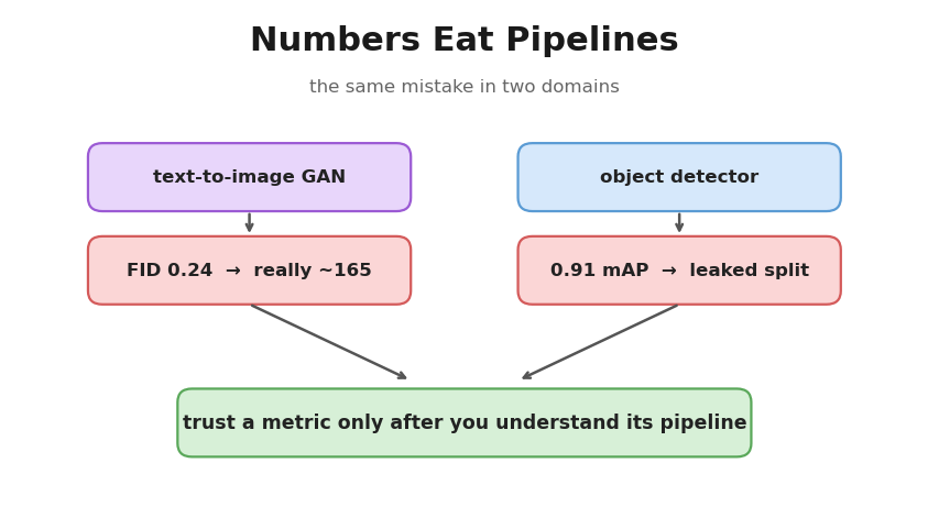
A detector reported 0.91 near-train mAP, a GAN reported a non-standard FID of 0.24, and a diffusion model's validation loss plateaued at 0.9425 -- the exact NLL of a two-scalar constant baseline. All three numbers were easy to overinterpret until their pipelines were audited.
The pattern
Three unrelated projects on this blog — a safety-gear object detector, a text-to-image GAN, and an image diffusion model — converged on the same lesson, the hard way. In each, the headline number looked impressive (or, for the diffusion model, looked converged) but did not support the conclusion initially attached to it. The fix began with a better understanding of what the number was made of.
- The detector scored 0.91 mAP. It also fired
helmet_offon workers wearing helmets. - The GAN scored FID 0.24 in a non-standard feature space. A canonical 2048-d re-evaluation on one N=510 draw was ~205.
- The diffusion model’s validation loss plateaued at 0.9425. That was the exact analytic NLL of the best constant two-scalar Gaussian — a 329,452,500-parameter network scoring like a two-parameter one.
None of these results was fabricated by the model. All three were pipeline-dependent measurements presented without enough scope — and the habit that caught that problem is portable across domains. This post pulls the three threads together and shows how a cheap experiment can reprioritize a hypothesis without pretending to prove its cause.
Failure mode #1 — a non-comparable generative metric
The GAN’s evaluation notebook computed FID with a library default that scored in the wrong feature space — 1000-d Inception logits instead of the conventional 2048-d pool3. The number it produced (0.24) was on a non-comparable scale; a canonical-extractor N=510 draw for the original model was ~205 (the ratio is model-dependent, so the two do not convert). That estimate is useful for same-N internal diagnosis, not a uniquely “real” or literature-comparable FID. The full diagnosis is here, and the reusable reporting protocol here.
The tell was a mismatch between the tiny number and visibly blurry samples. Published face-GAN ranges were a reason to audit the pipeline, not a direct benchmark because sample count and preprocessing differed. A number that contradicts every qualitative check needs an audit before celebration.
Failure mode #2 — a near-train detection split
The detector’s “held-out” validation split wasn’t held out the way it looked: AIHub’s official split interleaves frames within the same clip, so ~94% of validation frames sat within ±1 label-index of a training frame from the same fixed camera. The 0.91 was a near-train number. A second probe (false positives) overlapped the training negatives, and an unfixed seed blurred the small deltas. The self-audit is here.
Same shape as the first failure mode: the scalar could be computed correctly while answering the wrong deployment question. “Fakes from one fixed prompt” (a second FID sampling bug) and “validation frames from training clips” (the mAP split issue) both narrow the evaluated distribution without making that scope obvious.
Failure mode #3 — a converged loss that wasn’t
A public PyTorch reimplementation of Sohl-Dickstein et al. 2015 (arXiv:1503.03585) had its MNIST validation loss pinned at 0.9424–0.9426 for thousands of batches. A flat loss reads as convergence — until you compute what a trivial baseline costs on the same objective. Normalized to [-1, 1], MNIST test has global mean -0.7350 and std 0.6210; the analytic NLL of the best constant two-scalar Gaussian fit to that data is 0.9425. A 329,452,500-parameter model was matching a two-parameter baseline to four significant figures. The root cause: the forward posterior q(x^(t-1)|x^(t),x^(0)) — the term the paper’s entire training objective is built from — appeared nowhere in the image-model code path. The full audit is here.
Same smell as the other two, with a twist specific to this domain: the samples were visibly noise while the loss looked converged, and nobody caught it by eye because torchvision’s make_grid(normalize=True) min-max-stretches degenerate output to full contrast before rendering. A near-uniform noise tensor gets stretched until it looks like a normal-contrast image in TensorBoard — the rendering pipeline hid the failure exactly the way the wrong feature space hid the FID one.
The common law: numbers eat pipelines
A single-scalar metric is a compression of the truth, and the compression artifacts live in the pipeline that produced it — not in the scalar:
| generative (FID) | detection (mAP) | diffusion (val loss) | |
|---|---|---|---|
| headline | 0.24 (non-standard; canonical N=510 draw ~205) | 0.91 (near-train) | 0.9425 (equals a 2-scalar baseline) |
| where it broke | feature space + input pipeline | the train/val split (sampling) | the objective (missing forward posterior) + the sample rendering |
| the smell | “too good vs literature” | “too good vs reality (false positives)” | “converged vs visibly noisy samples” |
| the fix | pin extractor/pipeline/N | split by clip, disjoint probes, fixed seed | diff the reference implementation line by line; render with a fixed inverse mapping |
| reusable artifact | FID checklist | anti-fooling rules | difficulty ladder |
flowchart TD
    M["a single-number metric"] --> P["the pipeline behind it<br/>(features, resize, split, sampling, seed)"]
    P --> T["what the number actually measures"]
    H["the headline you report"] -.->|"only honest if"| T
The practical rule all three projects converged on: never quote a metric you have not tried to break. A same-tensor real-vs-real score near zero checks only the accumulator identity path; add independent splits and preprocessing perturbations. Split by the unit that leaks, check probe overlap by file hash, and use literature ranges only as audit triggers unless protocols match. The number is a claim; the pipeline is the evidence.
The other half: kill wrong hypotheses cheaply
Distrust applies to your explanations, not just your measurements. Once the GAN used the canonical feature definition, its historical N=510 estimates plateaued around ~160 and its losses suggested a tempting hypothesis: D may be too strong. The raw loss magnitudes were not themselves a calibrated dominance diagnostic.
So I tested it instead of assuming it: four single-seed configurations bundled EMA, separate learning rates, label smoothing, and reduced D-update frequency against a pre-registered decision rule. None robustly broke the baseline-equivalent band, which lowered the priority of those settings but did not reject D-dominance generally. A later single DiffAugment run produced a lower same-N estimate, 163 → 118.5; without repeated seeds or overfitting diagnostics, that supports a promising intervention rather than proving its mechanism.
The diffusion audit’s difficulty ladder is the same move again, run cheaper. Once the training objective was fixed, full-MNIST generation still came out as speckle, and the tempting hypothesis was “the sampler or architecture is still broken.” Training the larger model long enough for a fair verdict on full MNIST would have cost something like 14.6 GPU-hours – the 5M run’s 46,900 steps at the 46M model’s measured 1,124.4 ms/step train rate. Instead, the same image path was pointed at strictly easier data: synthetic disks produced solid but irregular blobs (0.000 mid-tone fraction, raw output std 0.593), a single MNIST class (“1”) produced correctly-oriented but fragmented strokes, and full MNIST alone stayed speckle. That reprioritized the hypothesis from “the sampler is broken” to “the data is harder than the training budget,” for roughly 35 minutes of compute. As with the D-dominance sweep, this is a prioritization result, not a causal proof — it makes one explanation more worth chasing first, not the only one left standing.
The economics still matter. A cheap screen can tell you whether to spend the next week on a direction, and the evaluation-leakage audit is the same move pointed inward: challenging your own evaluation is cheaper than having a reviewer or production challenge it for you. A causal rejection needs one-factor ablations, repeated seeds, uncertainty and mechanism-specific diagnostics; this sweep was a prioritization result, not that stronger experiment.
A portable discipline
Strip the domains away and the same checklist-of-checklists is left:
- Distrust the metric. Know what the scalar compresses; pin the pipeline; use same-set identity and independent-split controls; sanity-check against literature without claiming comparability. (FID / mAP versions.)
- Distrust the split. Split by the unit that leaks (clip, patient, scene), and verify disjointness by hash, not by name.
- Distrust the explanation. Pre-register a decision rule and use a cheap screen to reprioritize; change one variable and repeat seeds before making a causal rejection.
- Lead with the uncontaminated number, and label the rosier one with an asterisk.
None of this starts with a bigger GPU. It starts by treating the first number as provisional until its scope and failure modes have been tested.
Conclusion
The most useful thing I did across these projects was audit what each output meant: the FID that read 0.24, the near-train mAP that read 0.91, the diffusion loss that read 0.9425, and the “obvious” reason the GAN was stuck. Numbers eat pipelines. Measure the pipeline, not just the scalar, and design experiments that distinguish screening evidence from causal evidence. That habit transferred between a detector, a GAN, and a diffusion model with little else in common.
Resources
- Generative-metric thread — “Your FID of 0.24 Isn’t Near-Perfect” and the “FID reporting checklist”
- Detection-metric thread — “Held-Out in Name Only” (evaluation self-audit) and “When 0.91 mAP Still Fails”
- Diffusion-model thread — “Your Loss Converged. The Model Learned Two Numbers.”
- Cheap hypothesis screening — “Testing a Hypothesis Cheaply”
- Leakage, generally — Kaufman et al., Leakage in Data Mining (ACM TKDD, 2012) (ACM)